Expectation-Maximization

Expectation-Maximization [1] is a clustering algorithm which has an iterative approach. It basically computes maximum likelihood estimates iteratively and updates the distribution parameters (π, Σ, μ) according to this likelihood information. This update can be implemented according to the log-likelihood and log-posterior [2].

In this project, I implemented this solution to cluster a dataset which is a Gaussian Mixture model, includes 3 different Gaussian distribution.

For the full pipeline:

1. Finding the best parameters

We are trying to find best parameters theta (π, Σ, μ) to maximize the log-likelihood of each data to appropriate distribution (here we can think distribution as clusters) [3]. There is a paradox here. Since we don’t know the distributions from the beginning, we can not calculate the likelihood. Since we can not calculate the likelihood, we can not maximize it and find the appropriate Gaussian distributions of dataset.

To break this loop and start calculation, we determine random inital parameters for 3 Gaussian distributions: (π0, π1, π2, Σ0, Σ1, Σ2, μ0, μ1, μ2)

def random_sigma(n):
    x = np.random.normal(0, 1, size=(n, n))
    return np.dot(x, x.transpose())
def initialize_random_params():
    a = np.random.uniform(0, 1)
    b = np.random.uniform(0, 1)
    c = np.random.uniform(0, 1)
    sum_ = a + b + c
    params = {'phi0': a/sum_,
              'phi1': b/sum_,
              'phi2': c/sum_,
              'mu0': np.random.normal(0, 1, size=(2,)),
              'mu1': np.random.normal(0, 1, size=(2,)),
              'mu2': np.random.normal(0, 1, size=(2,)),
              'sigma0': random_sigma(2),
              'sigma1': random_sigma(2),
              'sigma2': random_sigma(2)}
    return params

2. Expectation

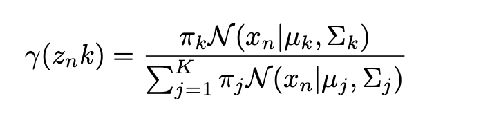
In this part, by using the parameters, I calculated the likelihoods of all the data points according to the different distributions. Than by using the formula down below, I calculated a posterior probability (sometimes people refer this responsibility) [4] for each of the data points and for each of the distributions. We will use this probabilities to update the parameters in maximization step.

def e_step(x, params):
    likelihood_0= stats.multivariate_normal(params["mu0"], params["sigma0"]).pdf(x)
    likelihood_1= stats.multivariate_normal(params["mu1"], params["sigma1"]).pdf(x)
    likelihood_2= stats.multivariate_normal(params["mu2"], params["sigma2"]).pdf(x)
    phi_0= params["phi0"]
    phi_1= params["phi1"]
    phi_2= params["phi2"]
    posterior_0= phi_0 * likelihood_0
    posterior_1= phi_1 * likelihood_1
    posterior_2= phi_2 * likelihood_2
    post_sum_=np.add(posterior_0, posterior_1)
    post_sum = np.add(post_sum_, posterior_2)
    probabilities_0 = np.divide(posterior_0,post_sum)
    probabilities_1 = np.divide(posterior_1,post_sum)
    probabilities_2 = np.divide(posterior_2,post_sum)
    avg_likelihood = np.array([np.mean(np.log(likelihood_0+0.0000001)), np.mean(np.log(likelihood_1+0.0000001)), np.mean(np.log(likelihood_2+0.0000001))])
    posteriors = np.array([probabilities_0,probabilities_1,probabilities_2])
    return avg_likelihood, probabilities_0, probabilities_1, probabilities_2, posteriors

3. Maximization

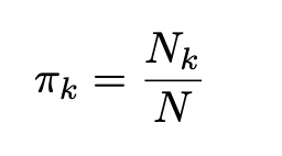
By using the probabilities come from the expectation step, we update the π, μ and Σ parameters in maximization step, to increase the each point’s likelihood to appropriate Gaussian distribution. Which also means to devide data points into clusters in most correct way. To update the πk values, we sum the probabilities which came for the kth distribution, and divide it by the total data point count.

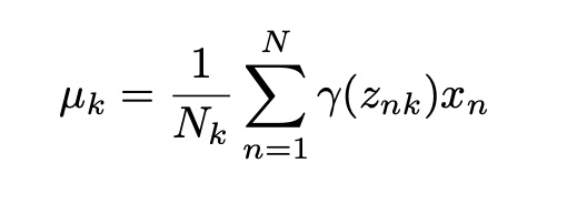
To update the μk values, we multiply the datapoints with their probabilities and sum. Then, we divide this sum to the sum of the probabilities.

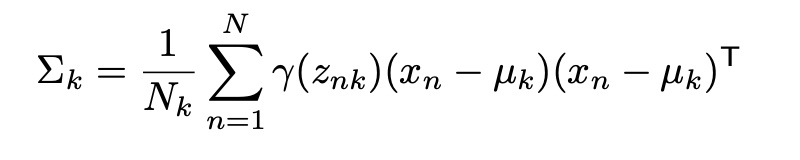
To update the Σ values, we first calculate the differences between the data points and the mean, and then multiply this difference, the transpose of this difference and the probabilities of these data points. And we divide this value to the sum of the probabilities.

We save the average likelihood of all points for all the distributions. As a convergence condition, we check the difference between this step’s value and previous step’s value. If the difference is smaller than ”0.0000001”, it means algorithm converged and code stops.

def m_step(x, params):
    total_count = x.shape[0]
    _ , prob0, prob1, prob2, posteriors = e_step(x, params)
    sum_prob0 = np.sum(prob0)
    sum_prob1 = np.sum(prob1)
    sum_prob2 = np.sum(prob2)
    phi0 = (sum_prob0 / total_count)
    phi1 = (sum_prob1 / total_count)
    phi2 = (sum_prob2 / total_count)
    mu0 = (prob0.T.dot(x)/sum_prob0).flatten()
    mu1 = (prob1.T.dot(x)/sum_prob1).flatten()
    mu2 = (prob2.T.dot(x)/sum_prob2).flatten()
    diff0 = x - mu0
    sigma0 = diff0.T.dot(diff0 * prob0[..., np.newaxis]) / sum_prob0
    diff1 = x - mu1
    sigma1 = diff1.T.dot(diff1 * prob1[..., np.newaxis]) / sum_prob1
    diff2 = x - mu2
    sigma2 = diff2.T.dot(diff2 * prob2[..., np.newaxis]) / sum_prob2
    params = {'phi0': phi0, 'phi1': phi1, 'phi2': phi2, 'mu0': mu0, 'mu1': mu1, 'mu2': mu2, 'sigma0': sigma0, 'sigma1': sigma1, 'sigma2': sigma2}
    return params

4. Results

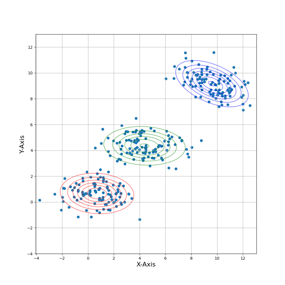
You can see the visualization of my solution in Figure 1. I found this solutions with 47 steps. The parameters I have found was: π0 = 0.33350133224135536
μ0 = [4.37904703 4.35183928]
Σ0 = [2.74789528 −0.1192322
−0.1192322 0.61806456]
π1 = 0.3331653516861432
μ1 = [0.70208295 0.6613623]
Σ1 = [2.11797378 −0.09973243
−0.09973243 0.64083765]
π2 = 0.33333331607250144
μ2 = [9.60515914 9.16835945]
Σ2 = [2.01245136 −0.64166751
−0.64166751 0.82171149]

5. References

In the script, I inspired by the blog here: https://towardsdatascience.com/implement-expectation-maximization-em-algorithm-in-python-from-scratch-f1278d1b9137
For the plotting part, I followed the same approach with this blog: https://medium.com/@prateek.shubham.94/expectation-maximization-algorithm-7a4d1b65ca55

[1] Dempster, A. P., N. M. Laird and D. B. Rubin, “Maximum Likelihood from Incomplete Data Via the EM Algorithm”, Journal of the Royal Statistical Society: Series B (Methodological), Vol. 39, No. 1, pp. 1–22, 1977, https://rss.onlinelibrary.wiley.com/doi/abs/10.1111/j.2517-6161.1977.tb01600.x.
[2] Dellaert, F., “The Expectation Maximization Algorithm”, , 07 2003.
[3] Moon, T. K., “The expectation-maximization algorithm”, IEEE Signal Processing Magazine, Vol. 13, No. 6, pp. 47–60, Nov 1996.
[4] Gebru, I. D., X. Alameda-Pineda, F. Forbes and R. Horaud, “EM Algorithms for Weighted-Data Clustering with Application to Audio-Visual Scene Analysis”, IEEE Transactions on Pattern Analysis and Machine Intelligence, Vol. 38, No. 12, pp. 2402–2415, Dec 2016.